Suppose $\mathbf{x} \sim p(X)$ is a random variable, and $y = f(\mathbf{X})$. In this section, we will find how to calculate $p(y)$.
Discrete Random Variable Case
If $\mathbf{X}$ is a discrete random variable, the pmf of $\mathbf{Y}$ is simply computed by summing the probability mass functions of the values $x$ such that $f(x) = y$.
$$ p_y(y) = \sum_{x: f(\mathbf{X}) = y} p_x(\mathbf{X}) \tag{1} $$
Continuous Random Variable Case
If $\mathbf{X}$ is a continuous random variable, $p_x(\mathbf{X})$ is a probability density function, so we cannot use formula (1). Instead, we will work with the cumulative distribution function (CDF), i.e., $P_x(\mathbf{x})$ and $P_y(y)$.
$$ P_y(y) \overset{\text{$\Delta$}}{=} Pr(Y \leq y) = Pr(f(\mathbf{X}) \leq y) = Pr(\mathbf{X} \in {x \mid f(\mathbf{x}) \leq y }) $$
Where:
- The CDF $P_y(y)$ gives the probability that the random variable $\mathbf{Y}$ (generated from $f(\mathbf{X})$) is less than or equal to $y$.
- In this case, we are calculating the probability that $f(\mathbf{X})$ is less than or equal to $y$ by finding all values of $x$ such that $f(\mathbf{X}) \leq y$, and then calculating the probability for these values of $x$.
If $f(x)$ is an invertible function, we can find $p_y(y)$ by differentiating the CDF. Otherwise, we need to use other approximation methods, such as Monte Carlo, to find the pdf $p_y(y)$.
Invertible Transformations (Bijections)
In this section, we focus on the cases of monotonic and invertible functions. A function is invertible if and only if it is a bijector (bijective).
The condition for a function $f: \mathbf{X} \to Y$ to be a bijector is when it has two properties:
- (a) Injective (one-to-one), meaning each distinct element in set $\mathbf{X}$ is mapped to a distinct element in set $Y$,
- (b) Surjective (onto), meaning each element in set $Y$ has at least one element in set $\mathbf{X}$ mapped to it.
Change of Variables: Scalar Case
We start with an example. Suppose $x \sim \text{Unif}(0, 1)$, and $y = f(x) = 2x + 1$. This function stretches and shifts the probability distribution, as illustrated in Fig.1 (a).
Now, zooming in on a point $x$ and a nearby point, more precisely, $x + dx$, we see that this interval is mapped to $(y, y + dy)$. The probability mass in these intervals must remain the same, so $p(x) dx = p(y) dy$, and thus:
$$ p_y(y) = p_x(x) \frac{dx}{dy} $$
However, since it doesn’t matter (in terms of probability conservation) whether $\frac{dx}{dy} > 0$ or $\frac{dx}{dy} < 0$, we have:
$$ p_y(y) = p_x(x)\left| \frac{dx}{dy} \right| $$
where:
- The derivative $\frac{dx}{dy}$ indicates the rate of change of $x$ with respect to $y$. This is a scaling factor that describes how the probability density changes when transforming from $x$ to $y$.
- When $\frac{dx}{dy}$ is large, the transformation from $y$ to $x$ makes the density $p_y(y)$ “thinner” compared to $p_x(x)$, and vice versa.
- The absolute value $\left| \frac{dx}{dy} \right|$ is used to ensure that the probability density is non-negative.
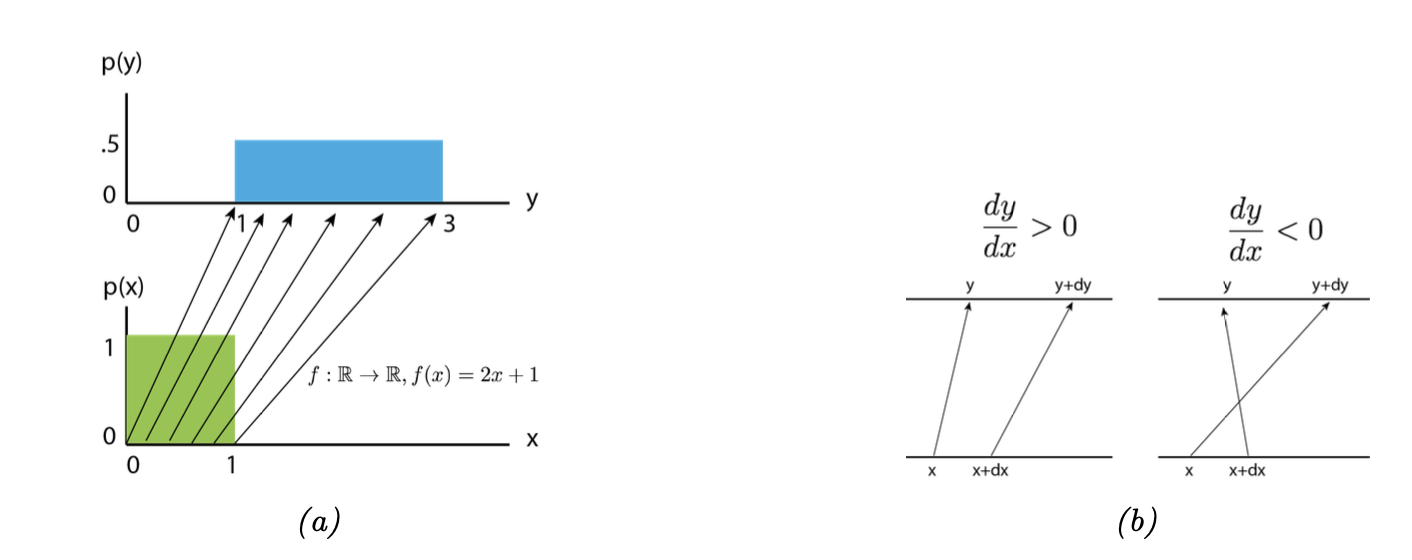
Fig.1
Now, let’s consider the general case for any $p_x(x)$ and any monotonic function $f: \mathbb{R} \to \mathbb{R}$. Let $g = f^{-1}$, so that $y = f(x)$ and $x = g(y)$. If we assume that $f: \mathbb{R} \to \mathbb{R}$ is monotonically increasing, we have:
$$ P_y(y) = \Pr(f(\mathbf{X}) \leq y) = \Pr(\mathbf{X} \leq g(y)) = P_x(g(y)) $$
Taking the derivative, we get:
$$ p_y(y) = \frac{d}{dy} P_y(y) = \frac{d}{dy} P_x(g(y)) = \frac{dx}{dy} \frac{d}{dx} P_x(g(y)) = \frac{dx}{dy} p_x(g(y)) $$
We can derive a similar expression (but with the opposite sign) for the case where $f$ is monotonically decreasing. To handle the general case, we take the absolute value to obtain:
$$ p_y(y) = p_x(g(y)) \left| \frac{d}{dy} g(y) \right| $$
This is known as the change of variables formula.
Change of Variables: Multivariable Case
We can extend the previous result to multivariable distributions as follows. Suppose $f$ is an invertible function mapping $\mathbb{R}^n$ to $\mathbb{R}^n$, with inverse $g$. Suppose we want to compute the pdf of $y = f(x)$. Similarly to the scalar case, we have:
$$ p_y(y) = p_x(g(y)) \left| \det [J_g(y)] \right| \tag{3} $$
where:
- $J_g = \frac{dg(y)}{dy^T}$ is the Jacobian of $g$, and $\left| \det J_g(y) \right|$ is the absolute value of the determinant of $J$ evaluated at $y$.
- The Jacobian is a matrix of partial derivatives, containing information on how each component of the vector $\mathbf{y}$ changes with respect to each component of the vector $\mathbf{x}$.
- The determinant of the Jacobian, $\det(\text{Jacobian})$, describes the transformation of “volume” (or area in 2D) when moving from the $\mathbf{x}$-space to the $\mathbf{y}$-space. This generalizes the concept of $\frac{dx}{dy}$ in the univariate case.
- The absolute value of the determinant $\left| \det(\text{Jacobian}) \right|$ represents the scaling factor between probability densities in the two spaces.
Consider the example of a coordinate change between Cartesian and polar coordinates. Here, $x = (x_1, x_2)$, $y = f(x) = f(x_1, x_2) = (r, \theta)$, and $g(y) = f^{-1}(y) = f^{-1}(r, \theta) = (r\cos\theta, r\sin\theta)$.
Applying equation (3), we have:
$$ p_{r, \theta}(r, \theta) = p_{x_1, x_2}(r\cos\theta, r\sin\theta) \left| \det [J_g(y)] \right| \tag{4} $$
where:
$$ \mathbf{J}_g = \begin{bmatrix} \frac{\partial x_1}{\partial r} & \frac{\partial x_1}{\partial \theta} \ \frac{\partial x_2}{\partial r} & \frac{\partial x_2}{\partial \theta} \end{bmatrix} = \begin{bmatrix} \cos\theta & -r\sin\theta \ \sin\theta & r\cos\theta \end{bmatrix} \Rightarrow |\text{det}(\mathbf{J}_g)| = |r\cos^2\theta + r\sin^2\theta| = |r| $$
Thus, equation (4) becomes:
$$ p_{r, \theta}(r, \theta) = p_{x_1, x_2}(r\cos\theta, r\sin\theta) |r| \tag{5} $$
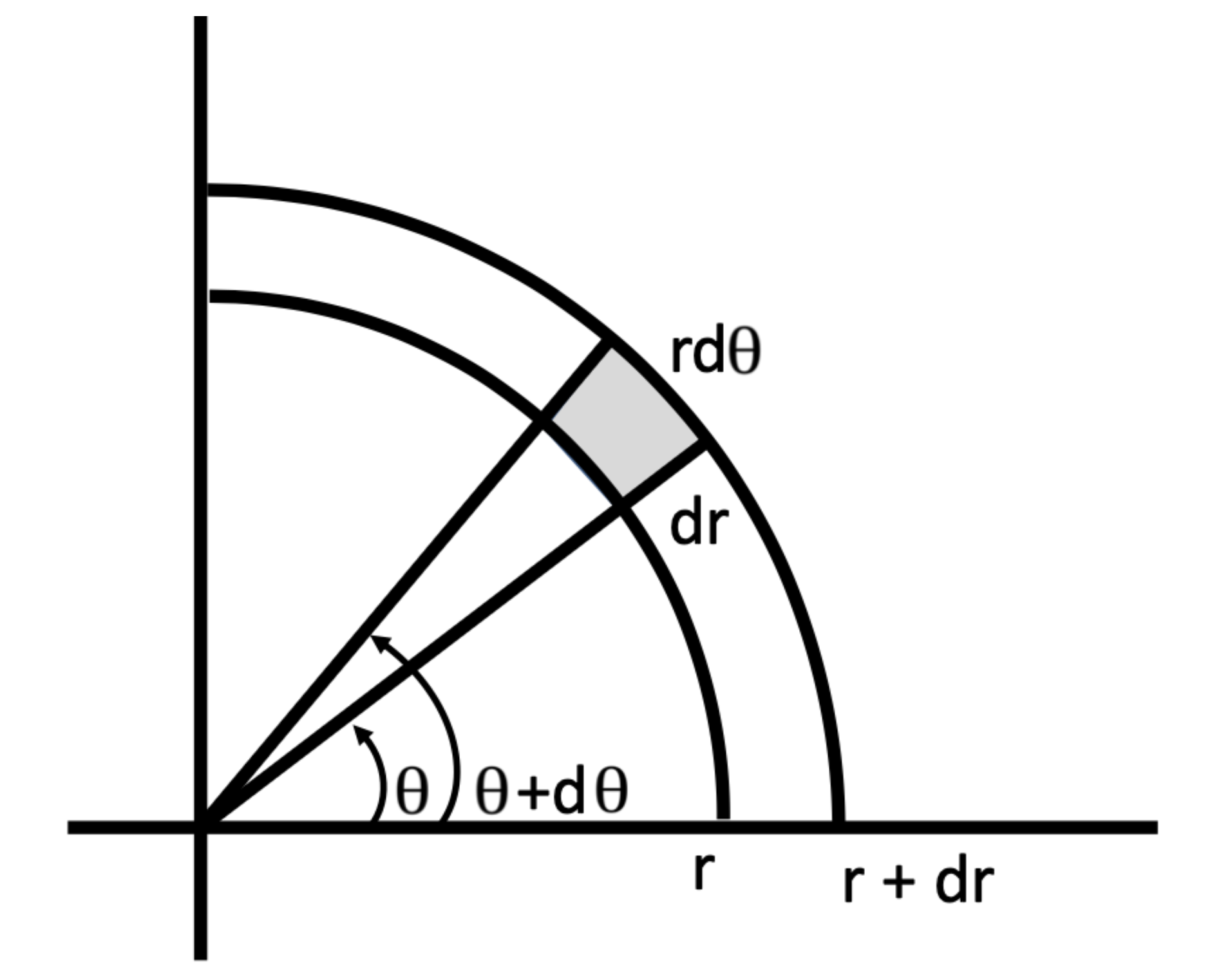
Fig. 2
The area of the shaded region in the figure is $r dr d\theta$. The probability of a point falling in the shaded region is:
$$ \Pr(r \leq \mathbf{R} \leq r+dr, \theta \leq \Theta \leq \theta + d\theta) = p_{r, \theta}(r, \theta) dr d\theta \tag{6} $$
where $\text{VT}$ is the probability of a point falling within a small region in the polar coordinate system, defined by $r$ and $\theta$. To prove the VP of equation (6), we need to rewrite it as an integral:
$$ \begin{align*} \Pr(r \leq \mathbf{R} \leq r+dr, \theta \leq \Theta \leq \theta + d\theta) &= \int_{\theta}^{\theta+d\theta} \int_{r}^{r+dr} p_{r, \theta}(r, \theta)dr d\theta \end{align*} \tag{6.1} $$
Here, $p_{r, \theta}(r, \theta)$ is the probability density function of a point near $(r, \theta)$. Since the region $dr$ and $d\theta$ is very small, we treat the density function as constant within that region, simplifying the integral.
Thus, the VP of equation (6.1) can be rewritten as:
$$ \begin{align*} \Pr(r \leq \mathbf{R} \leq r+dr, \theta \leq \Theta \leq \theta + d\theta) &= p_{r, \theta}(r, \theta) \int_{\theta}^{\theta+d\theta} \int_{r}^{r+dr} dr d\theta \ &= p_{r, \theta}(r, \theta) dr d\theta \tag{cmx} \end{align*} $$
Applying the change of variables to equation (6), we get:
$$ p_{r, \theta}(r, \theta) dr d\theta = p_{x_1, x_2}(r\cos\theta, r\sin\theta) r dr d\theta \tag{7} $$
In other words, in the limit as $dr$ and $d\theta$ become infinitesimally small, the change in the density function within this region can be ignored, and we only need to consider the value of the density function at a single point (the center of the region) to compute the probability.
The Convolution Theorem
Suppose $y = x_1 + x_2$, where $x_1$ and $x_2$ are independent random variables.
If these are discrete random variables, we can compute the probability mass function (pmf) for the sum as follows:
$$
p(y = j) = \sum_k p(x_1 = k)p(x_2 = j - k) \tag{8}
$$
where $j = \dots, -2, -1, 0, 1, 2, \dots$.
If $x_1$ and $x_2$ have probability density functions $p_1(x_1)$ and $p_2(x_2)$, what is the distribution of $y$? The cumulative distribution function (CDF) is given by:
$$ P_y(y^*) = \Pr(y \leq y^*) = \int_{-\infty}^{\infty} p_1(x_1) \left[ \int_{-\infty}^{y^*-x_1} p_2(x_2) , dx_2 \right] dx_1 \tag{9} $$
To find the PDF $p(y)$, we take the derivative of $P_y(y^*)$ with respect to $y^*$, and then substitute $y^* = y$.
Step 1:
- Take the derivative with respect to $y^*$. We have: $p(y) = \frac{d}{dy^*} P_y(y^*) \bigg|_{y^*=y}$.
- Substitute $P_y(y^*)$ from equation (9) into the expression:
$$ p(y) = \frac{d}{dy^*} \left( \int_{-\infty}^{\infty} p_1(x_1) \left[ \int_{-\infty}^{y^*-x_1} p_2(x_2) , dx_2 \right] dx_1 \right) $$ - Here, we need to differentiate the double integral with respect to $y^*$.
Step 2:
- Use the rule for differentiating under the integral sign:
$$ \frac{d}{dy^*} \int_{a(y^*)}^{b(y^*)} f(x) , dx = f(b(y^*)) \cdot \frac{db(y^*)}{dy^*} - f(a(y^*)) \cdot \frac{da(y^*)}{dy^*} $$ - In this case, $b(y^*) = y^* - x_1$, $a(y^*) = -\infty$, and $f(x_2) = p_2(x_2)$. Notice that:
$$ \frac{d}{dy^*} (y^* - x_1) = 1 - \frac{d}{dy^*} (-\infty) = 0 $$ - Therefore, the derivative of the integral in (9) with respect to $y^*$ is:
$$ \frac{d}{dy^*} \left( \int_{-\infty}^{y^*-x_1} p_2(x_2) , dx_2 \right) = p_2(y^* - x_1) \cdot 1 = p_2(y^* - x_1) $$
- Use the rule for differentiating under the integral sign:
Step 3:
- Substitute the result into the expression and simplify. After differentiating, substitute $y^* = y$:
$$ p(y) = \int_{-\infty}^{\infty} p_1(x_1) p_2(y - x_1) , dx_1 \tag{10} $$
This formula can be written as $p = p_1 \ast p_2$.
Here, $\ast$ represents the convolution operator. For vectors with finite length, the integrals become sums, and convolution can be seen as a flip-and-drag operation (Table 2.4).
Therefore, equation (10) is called the convolution theorem.
- Substitute the result into the expression and simplify. After differentiating, substitute $y^* = y$:
For example, suppose we roll two dice, so $p_1$ and $p_2$ are both uniform discrete distributions on the set ${1, 2, \dots, 6}$.
Let $y = x_1 + x_2$ be the sum of the two dice faces. We have:
$$ \begin{align*} p(y = 2) &= p(x_1 = 1)p(x_2 = 1) \\ &= \frac{1}{6} \times \frac{1}{6} \\ &= \frac{1}{36} \end{align*} $$
$$ \begin{align*} p(y = 3) &= p(x_1 = 1)p(x_2 = 2) + p(x_1 = 2)p(x_2 = 1) \\ &= \frac{1}{6} \times \frac{1}{6} + \frac{1}{6} \times \frac{1}{6} \\ &= \frac{2}{36} \end{align*} $$
Continuing this way, we find $p(y = 4) = 3/36$, $p(y = 5) = 4/36$, $p(y = 6) = 5/36$, $p(y = 7) = 6/36$, $p(y = 8) = 5/36$, $p(y = 9) = 4/36$, $p(y = 10) = 3/36$, $p(y = 11) = 2/36$, and $p(y = 12) = 1/36$. Figure 2.22 shows that the distribution looks like a Gaussian distribution.
We can also calculate the PDF of the sum of two continuous random variables. For example, in the case of Gaussian distributions, when $x_1 \sim \mathcal{N}(\mu_1, \sigma_1^2)$ and $x_2 \sim \mathcal{N}(\mu_2, \sigma_2^2)$, we can prove that if $y = x_1 + x_2$, then
$$ p(y) = \mathcal{N}(x_1|\mu_1, \sigma_1^2) \ast \mathcal{N}(x_2|\mu_2, \sigma_2^2) = \mathcal{N}(y|\mu_1 + \mu_2, \sigma_1^2 + \sigma_2^2) $$
Thus, the convolution of two Gaussian distributions is a Gaussian distribution.
Central Limit Theorem
Now, consider $N$ random variables with probability density functions $p_n(x)$ (not necessarily Gaussian), each having mean $\mu$ and variance $\sigma^2$.
We assume that each variable is independent and identically distributed (iid).
$$ X_n \sim p(X) $$
are independent samples from the same distribution. Let $S_N = \sum_{n=1}^{N} X_n$ be the sum of the random variables. It can be proven that as $N$ increases, the distribution of this sum approaches:
$$ p(S_N = u) = \frac{1}{\sqrt{2\pi N\sigma^2}} \exp\left(-\frac{(u - N\mu)^2}{2N\sigma^2}\right) $$
Thus, the distribution of the quantity
$$ Z_N \triangleq \frac{S_N - N\mu}{\sigma\sqrt{N}} = \frac{\overline{X} - \mu}{\sigma/\sqrt{N}} $$
converges to the standard normal distribution, where $\overline{X} = S_N/N$ is the sample mean. This is known as the Central Limit Theorem.
In Fig. 3, there is an example where the sample mean of random variables drawn from a Beta distribution is computed.
We see that the sample distribution of the mean quickly converges to a Gaussian distribution.
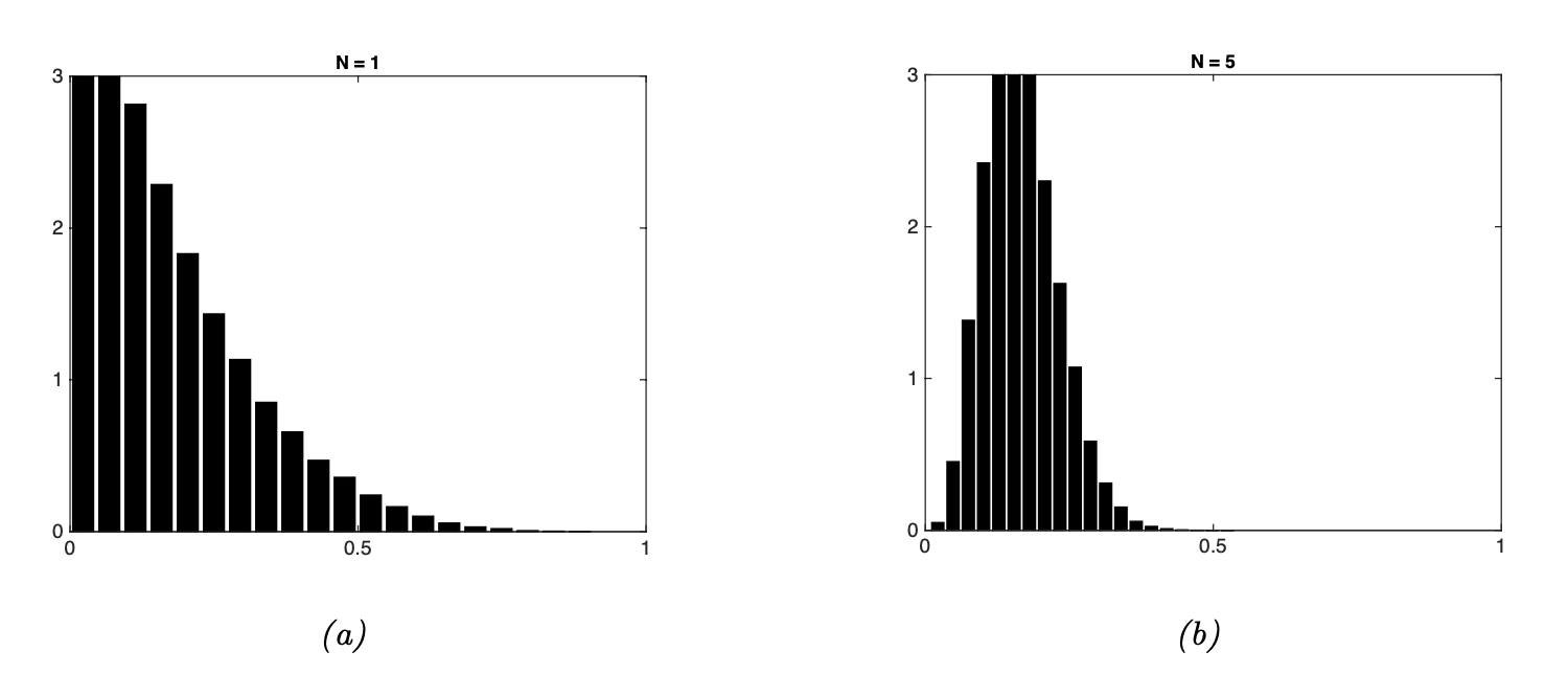
Fig. 3
Monte Carlo
Suppose $x$ is a random variable, and $y = f(x)$ is a function of $x$.
It is often difficult to compute the distribution $p(y)$.
A simple yet powerful method is to take a large number of samples from the distribution of $x$, and then use these samples (instead of the distribution) to approximate $p(y)$.
For example, suppose $x \sim \text{Unif}(-1, 1)$ and $y = f(x) = x^2$.
We can approximate $p(y)$ by taking many samples from $p(x)$ (using a uniform random number generator), squaring them, and calculating the empirical distribution of the results, given by:
$$ p_S(y) \triangleq \frac{1}{N_s} \sum_{s=1}^{N_s} \delta(y - y_s) \tag{2.179} $$
This method is essentially a “sum of Dirac deltas” with equal weights, each delta concentrated on one of the samples (2.7.6). By using enough samples, we can approximate $p(y)$ quite well $(Fig. 4)$.
This method is called the Monte Carlo approximation for the distribution.
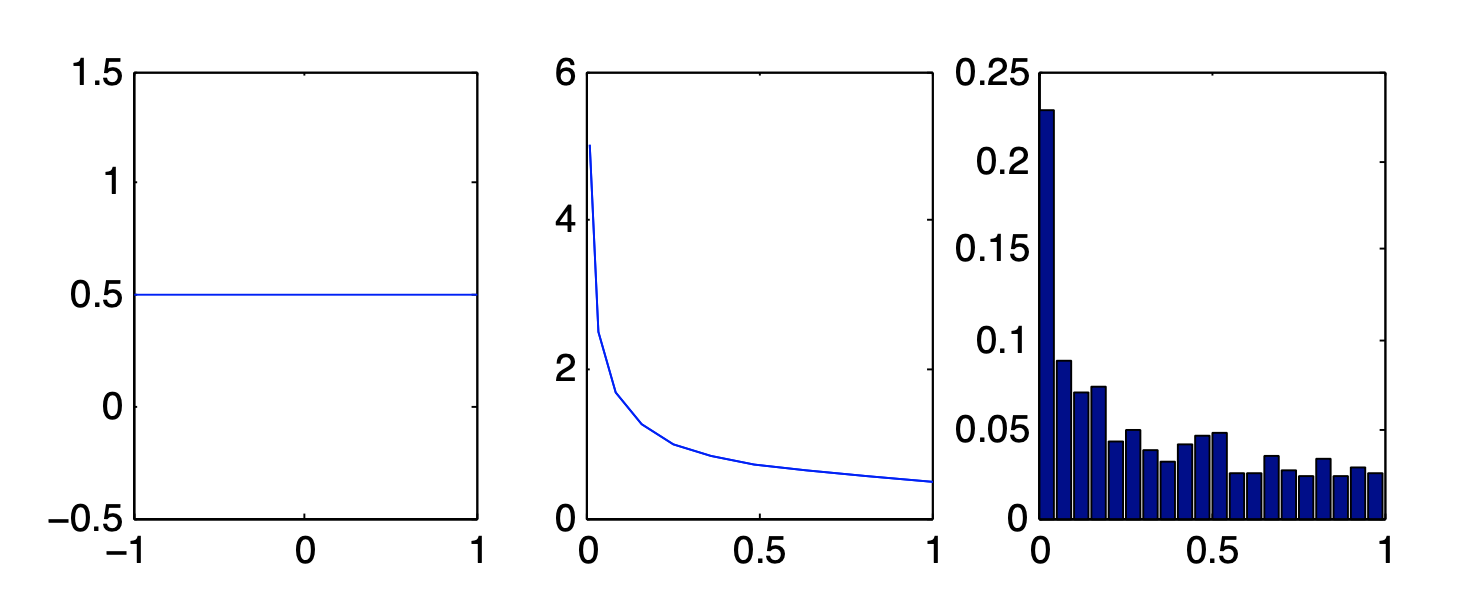
Fig. 4