Basic concepts in Linear Algebra
Scalar
A scalar is a single number.
In linear algebra, when referring to a scalar, we denote it with lowercase letters and describe which set the scalar belongs to. For example, $s \in \mathbf{R}$ indicates that $s$ is a real number, or $n \in \mathbf{N}$ indicates that $n$ is a natural number.
Vector
A vector is an array of numbers.
The numbers are arranged in a specific order, and we can use indices to access each number in the vector.
For example, $x_1$, $x_2$ respectively denote the first and second elements in the vector $\mathbb{x}$. Vectors are denoted by lowercase bold letters, such as $\mathbb{x}$. The elements in a vector are written in italic and accompanied by ordinal numbers, such as $x_1$, $x_2$.
When referring to a vector, we also need to know the type of values stored in it. If vector $\mathbb{x}$ has $n$ elements belonging to the set of real numbers $\mathbf{R}$, then vector $\mathbb{x} \in \mathbf{R}^n$. $\mathbf{R}^n$ is a vector space.
For example, $$ \mathbb{x} = \begin{bmatrix} 1 \\ 2 \\ 3 \end{bmatrix} $$
$\mathbb{x}$ has 3 elements, so $\mathbb{x} \in \mathbf{R}^3$.
Specifically, $\mathbb{x}$ is a point in the space $\mathbf{R}^3$. The coordinates of that point are determined by the values of the elements in $\mathbb{x}$. This means that, in the 3D space $Oxyz$, $\mathbb{x}$ will be located at the point with coordinates $x = 1, y = 2, z = 3$.
Operations on Vectors
Addition and Scalar Multiplication
When working with vectors, we have two operations: adding two vectors and multiplying a vector by a scalar.
$$ \begin{bmatrix} 1 \\ 2 \end{bmatrix} + \begin{bmatrix} 2 \\ 1 \end{bmatrix} = \begin{bmatrix} 3 \\ 3 \end{bmatrix} $$
$$ \begin{aligned} 2 \begin{bmatrix} 2 \\ 3 \end{bmatrix} = \begin{bmatrix} 4 \\ 6 \end{bmatrix} \end{aligned} $$
Addition of two vectors
Looking at the above figure, you might still not understand why there is a green vector in the middle. In fact, vector addition is tail-to-head, meaning you simply attach the head of one vector to the tail of the other vector.
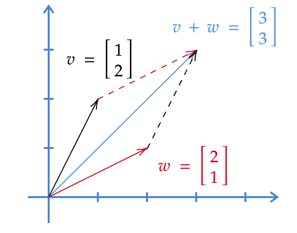
Extended vector addition
Let $u = v + w$ the resulting vector of the addition operation. $u$ represents a point in the 2D plane $Oxy$ with coordinates $x = 3$ and $y = 3$.
$$ \begin{aligned} \begin{bmatrix} 3 \\ 3 \end{bmatrix} = \begin{bmatrix} 3 \\ 0 \end{bmatrix} + \begin{bmatrix} 0 \\ 3 \end{bmatrix} \end{aligned} $$
Length of a vector
In high school, we learned how to calculate the length of a vector. The length of vector $u$ is the distance from point $v$ to the origin $O$ $(0, 0)$. Therefore, we can also say that vector $u$ represents an arrow with its tail at $(0, 0)$. That’s why in the addition operation above, we represent the resulting vector $u$ as an arrow from the origin to the point $(3, 3)$.
To compute the length of vector $u$, we take the square root of the sum of squares of its components:
$$ |u| = \sqrt{u_1^2 + u_2^2} $$
This is called the norm operation.
The norm is a function $| \cdot |$ that maps a point in the vector space $V$ to the real space $\mathbf{R}$ and satisfies the following properties:
- $| x | \ge 0$, with equality if and only if $x = 0$
- $| \alpha x | = |\alpha| | x |$
- $|x + y| \ge |x| + |y|$
for all $x, y \in V$ and $\alpha \in \mathbf{R}$.
Essentially, this operation calculates the distance between vector $u$ and vector $0$. Moreover, it is used to determine the distance between any two vectors $v$ and $w$ if $u = v - w$. To find the distance between two vectors, we apply the norm operation to the difference vector of those two vectors.
$$ \begin{aligned} d(v, w) = | v - w | \end{aligned} $$
Calculating the distance between two vectors is essential because it forms the basis for considering whether those two vectors are close or not. In certain fields such as machine learning, computing the distance between multi-dimensional vectors is a way to evaluate systems.
There are many types of norms, among which the most commonly used are the $l1$-norm (Manhattan distance) and the $l2$-norm (Euclidean distance).
$$ \begin{aligned} | x |_1 & = \sum_{i=1}^{n} |x_i| \\ | x |_2 & = \sum_{i=1}^{n} \sqrt{|{x_i}|^{2}} \\ | x |_p & = \Big( \sum_{i=1}^{n} |x_i|^p \Big)^{\frac{1}{p}}, \quad \forall p \ge 1 \end{aligned} $$
Matrix
A matrix is a data structure similar to a vector, but a matrix is a 2D array, so when accessing elements in it, we use 2 indices instead of 1 like in a vector. Matrices are usually denoted by uppercase letters and bolded.
A matrix ${A}$ with $m$ rows and $n$ columns is said to have a size of $m \times n$. Furthermore, if $A$ contains elements belonging to the set of real numbers $\mathbf{R}$, then we say $A \in \mathbf{R}^{m \times n}$.
Since each element in $A$ requires 2 indices to locate, the order of writing the indices of the elements follows the order of rows before columns. $A_{1,1}$ refers to the first element (leftmost of the first row) of $A$.
$$ \begin{aligned} \begin{bmatrix} A_{1,1} & A_{1,2} \\ A_{2,1} & A_{2,2} \end{bmatrix} \end{aligned} $$
So we can view a vector as a matrix with only 1 column, meaning if vector $\mathbb{x} \in \mathbf{R}^n$, then $\mathbb{x}$ is a matrix with a size of $n \times 1$.
We have an important operation applied to matrices, which is the transpose operation.
The matrix $A^T$ is the transpose of $A$ where the rows of $A^T$ are the columns of $A$ and vice versa.
$$ \begin{aligned} A = \begin{bmatrix} A_{1,1} & A_{1,2} & A_{1,3} \\ A_{2,1} & A_{2,2} & A_{2,3} \end{bmatrix} \rightarrow A^T = \begin{bmatrix} A_{1,1} & A_{2,1} \\ A_{1,2} & A_{2,2} \\ A_{1,3} & A_{2,3} \end{bmatrix} \end{aligned} $$
A scalar can also be viewed as a matrix with a size of $1 \times 1$. In that case, $a = a^T$.
Linear Combinations
A linear combination is the combination of two operations: addition and multiplication.
For $v, w$ being two vectors, $c, d$ being numbers, we have a linear combination as $cv + dw$.
Linear combination is a very important concept and can be considered a focal point in this subject. In the following lessons, you will see linear combinations being used continuously.
$$ \begin{aligned} 2 \begin{bmatrix} 2 & 2 \\ 1 & 1 \end{bmatrix} + 3 \begin{bmatrix} 1 & 2 \\ 3 & 4 \end{bmatrix} & = \begin{bmatrix} 7 & 10 \\ 11 & 14 \end{bmatrix} \end{aligned} $$
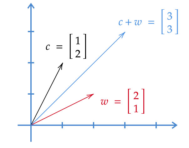
$\begin{bmatrix} 7 & 10 \\ 11 & 14 \end{bmatrix}$ is a linear combination with $c = 2$ and $d = 3$. For each pair of numbers $c, d$, we have a linear combination. The addition $w + v$ is also a linear combination with $c = d = 1$.
Linear combinations with $cv + dw$ with $v, w$ being two-dimensional vectors all lie in the $Oxy$ space. If $v, w$ have the form $\begin{bmatrix} a \\ b \\ c \end{bmatrix}$ ($v, w \in \mathbf{R}^3$), linear combinations $cv + dw$ lie in a plane belonging to the $Oxyz$ space. If we have an additional three-dimensional vector $u$, then the linear combination $cv + dw + eu$ lies in the entire $Oxyz$ space.
Today’s lesson is very concise, I only introduced the basic concepts in linear algebra and what we often use. In summary, we need to grasp the following concepts:
A vector of $n$ dimensions contains $n$ elements.
A vector can be seen as a representation of an arrow from the origin (see figure 2), a set of $n$ numbers, or a point in a plane.
We can add two vectors and multiply a vector by a number.
For two vectors $v$ and $w$, their linear combination is $cv + dw$.
Every linear combination $cv$ forms a line passing through the origin $(0, 0, 0)$.
Every linear combination $cv + dw$ forms a plane belonging to the three-dimensional space and passing through the origin $(0, 0, 0)$.
Every linear combination $cv + dw + eu$ forms a three-dimensional space.